Read in the FEMA National Risk Estimate table and split out by disaster
Author
Alan Jackson
Published
April 28, 2025
Read in the National Risk Estimates
Data downloaded from https://hazards.fema.gov/nri/data-resources#csvDownload
This is more painful than it sounds. The csv file has 467 columns, most of which are double precision, but some are character. And many are blank near the top of the file, so automatic schemes fail. Also, the number of columns for each disaster type varies, so simple schemes for determining how to read the data in will fail.
After (finally) getting it read in, I’ll look at it and then save files by disaster.
Metadata
The disaster codes are pretty easy to guess, but here are the definitions:
Hazard
Prefix
Avalanche
AVLN
Coastal Flooding
CFLD
Cold Wave
CWAV
Drought
DRGT
Earthquake
ERQK
Hail
HAIL
Heat Wave
HWAV
Hurricane
HRCN
Ice Storm
ISTM
Landslide
LNDS
Lightning
LTNG
Riverine Flooding
RFLD
Strong Wind
SWND
Tornado
TRND
Tsunami
TSUN
Volcanic Activity
VLCN
Wildfire
WFIR
Winter Weather
WNTW
Suffix
Meaning
EVNTS
Number of Events
AFREQ
Annualized Frequency
EXPB
Exposure - Building Value
EXPP
Exposure - Population
EXPPE
Exposure - Population Equivalence
EXPA
Exposure - Agriculture Value
EXPT
Exposure - Total
EXP_AREA
Exposure - Impacted Area (sq mi)
HLRB
Historic Loss Ratio - Buildings
HLRP
Historic Loss Ratio - Population
HLRA
Historic Loss Ratio - Agriculture
HLRR
Historic Loss Ratio - Total Rating
EALB
Expected Annual Loss - Building Value
EALP
Expected Annual Loss - Population
EALPE
Expected Annual Loss - Population Equivalence
EALA
Expected Annual Loss - Agriculture Value
EALT
Expected Annual Loss - Total
EALS
Expected Annual Loss Score
EALR
Expected Annual Loss Rating
ALRB
Expected Annual Loss Rate - Building
ALRP
Expected Annual Loss Rate - Population
ALRA
Expected Annual Loss Rate - Agriculture
ALR_NPCTL
Expected Annual Loss Rate - National Percentile
RISKV
Hazard Type Risk Index Value
RISKS
Hazard Type Risk Index Score
RISKR
Hazard Type Risk Index Rating
“Population Equivalence” is the monetary value of the exposed population, using a “value of statistical life (VSL)” approach.
Each fatality or ten injuries is treated as $11.6 million of economic loss.
Code
library(tidyverse)library(sf)library(leaflet)library(gt)googlecrs <-"EPSG:4326"path <-"/home/ajackson/Dropbox/Rprojects/ERD/Data/FEMA_National_Risk_Index_Data/"Datapath <-"/home/ajackson/Dropbox/Rprojects/Curated_Data_Files/"df <-read_csv(paste0(path, "NRI_Table_CensusTracts/NRI_Table_CensusTracts.csv"))foo <-names(df)[41:466] # only look at disaster categories# are all disasters the same? No.str_sub(foo, 1, 4) %>%as_tibble() %>%count(value) %>%gt() %>%tab_header(title=md("**Count of Fields for each Disaster**") ) %>%fmt_number(columns=n,sep_mark=',',decimals=0 ) %>%cols_label(value ="Disaster Code",n ="Number of Fields" )
Count of Fields for each Disaster
Disaster Code
Number of Fields
AVLN
22
CFLD
22
CWAV
26
DRGT
16
ERQK
22
HAIL
26
HRCN
26
HWAV
26
ISTM
22
LNDS
22
LTNG
22
RFLD
26
SWND
26
TRND
26
TSUN
22
VLCN
22
WFIR
26
WNTW
26
Code
# Build a table to decide how to read columnCspec <-str_extract(foo, "_.*") %>%as_tibble() %>%count(value)foo2 <- foo %>%as_tibble() %>%mutate(Spec=if_else(str_detect(value, "R$"), "c", "d"))Spec <-paste0(foo2$Spec, collapse="")Col_spec=paste0(str_dup("c",11), "ddddddcddcddddddddddddcddcddd", Spec, "c")# Try againdf <-read_csv(paste0(path, "NRI_Table_CensusTracts/NRI_Table_CensusTracts.csv"),col_types = Col_spec)
Let’s check for understanding and consistency
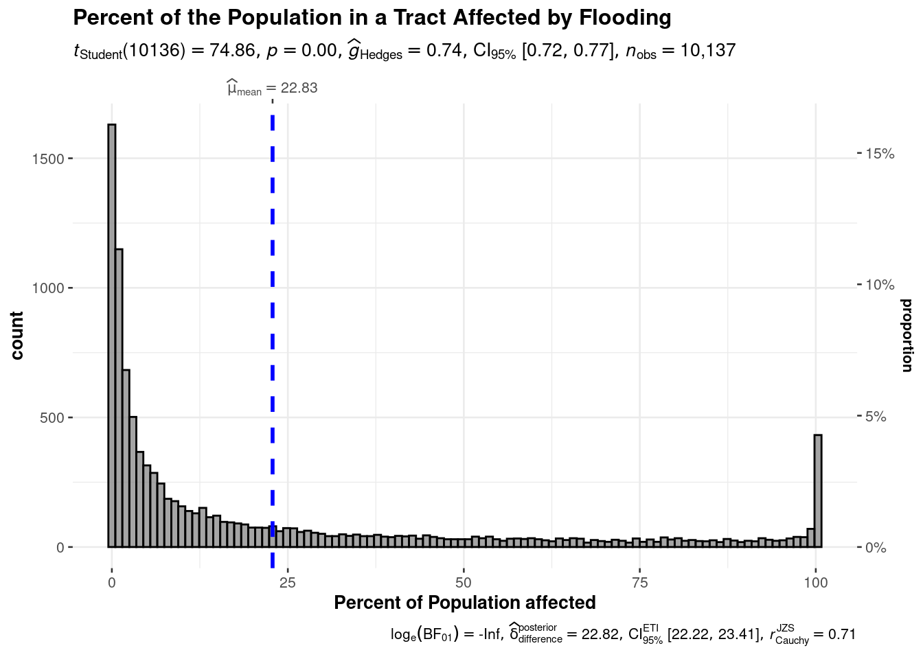
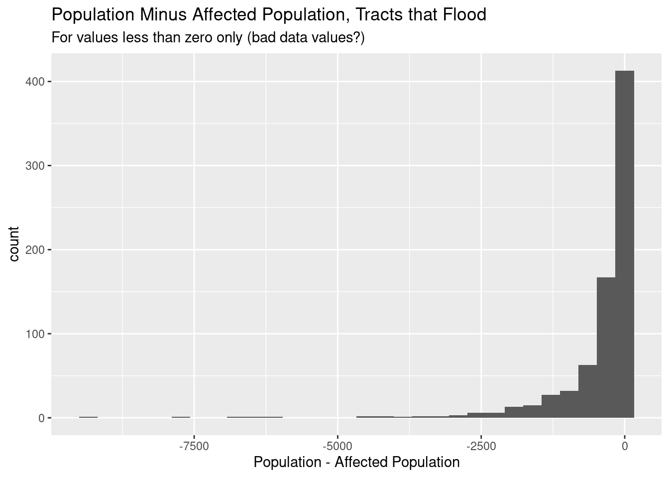
Hmmm… there are tracts where the number of people expected to be affected by the disaster is larger than the population of the tract.
Code
foo <- df %>%select(TRACTFIPS, POPULATION, CFLD_EXPP) %>%mutate(Pop_diff=(POPULATION - CFLD_EXPP)/POPULATION) %>%filter(Pop_diff>0) %>%filter(Pop_diff<1) %>%mutate(Pct_effected=CFLD_EXPP*100/POPULATION) ggstatsplot::gghistostats(data=foo,x=Pct_effected,xlab ="Percent of Population affected",title ="Percent of the Population in a Tract Affected by Flooding",subtitle ="After elimination of unrealistic values")
Code
df %>%select(TRACTFIPS, POPULATION, CFLD_EXPP) %>%mutate(Pop_diff=POPULATION - CFLD_EXPP) %>%filter(Pop_diff<0) %>%ggplot(aes(x=Pop_diff)) +geom_histogram() +labs(title="Population Minus Affected Population, Tracts that Flood",subtitle="For values less than zero only (bad data values?)",x="Population - Affected Population")
Attach the polygons and make a map
To highlight the more interesting areas, I will map only the tracts denoted by a risk rating of “very high”.
I’ll also restrict the data to tracts with a population of greater than 100, and with a percent of the population at flood risk greater than 25%.
Not surprisingly, most of the flood risk falls near the coast.
Code
df$RISK_RATNG %>%as_tibble() %>%count(value) %>%gt() %>%tab_header(title=md("**Count of Tracts for each Risk Rating**") ) %>%fmt_number(columns=n,sep_mark=',',decimals=0 ) %>%cols_label(value ="Risk Rating",n ="Number of Tracts" )
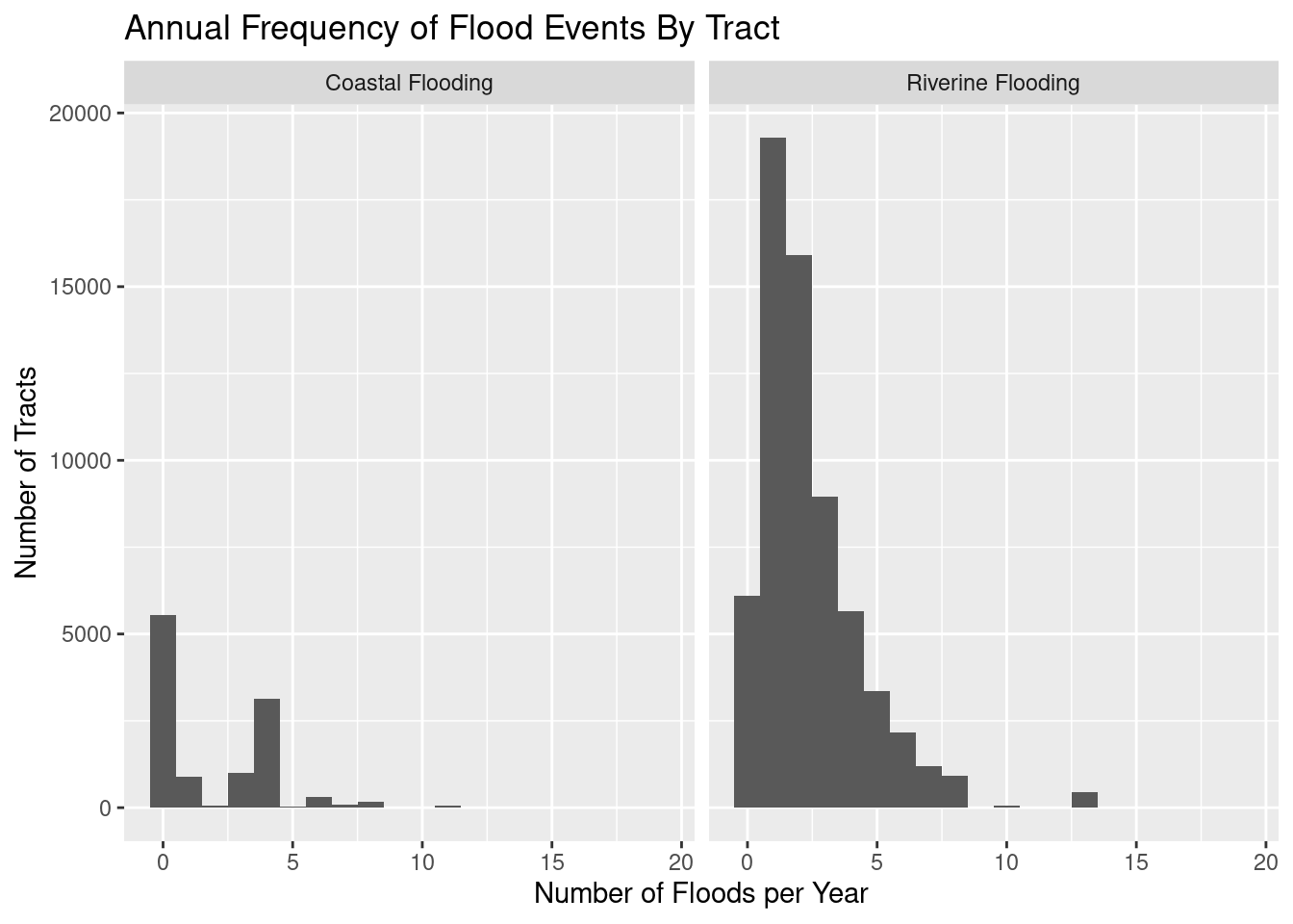
We’ll look at Coastal Flooding and Riverine Flooding
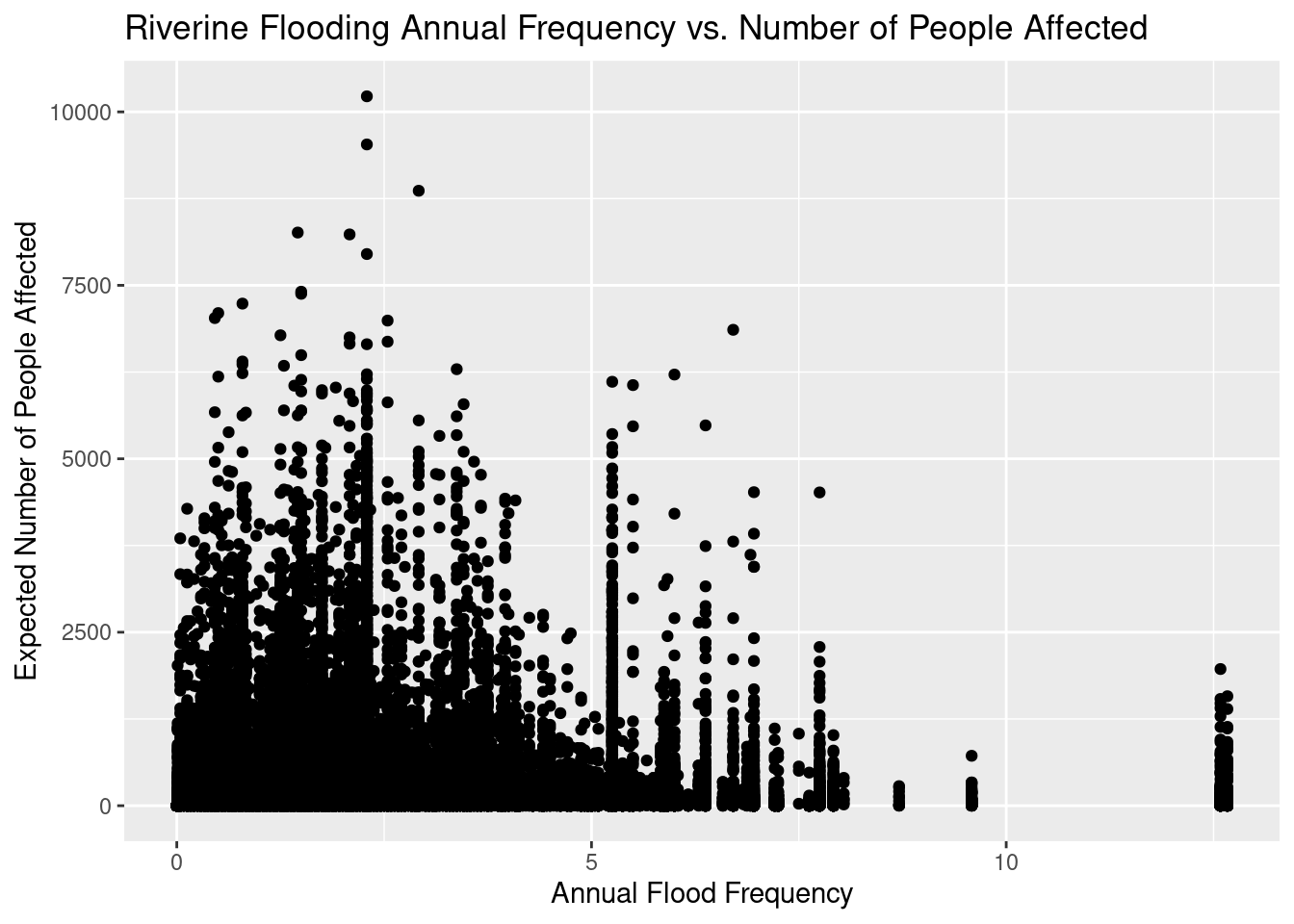
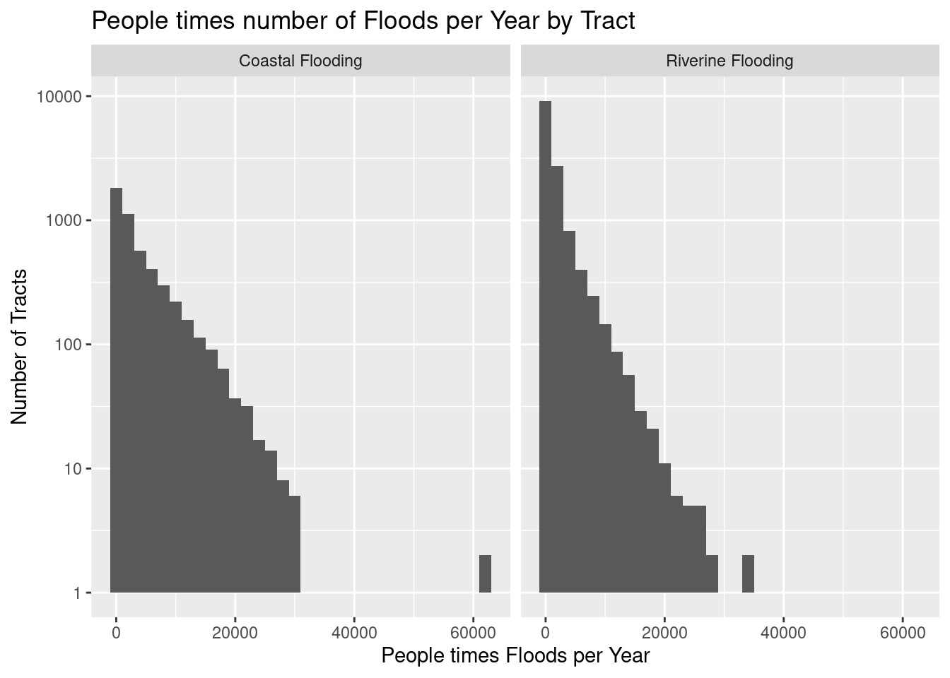
Many more tracts subject to river flooding, but coastal flooding has more potential to affect more people.
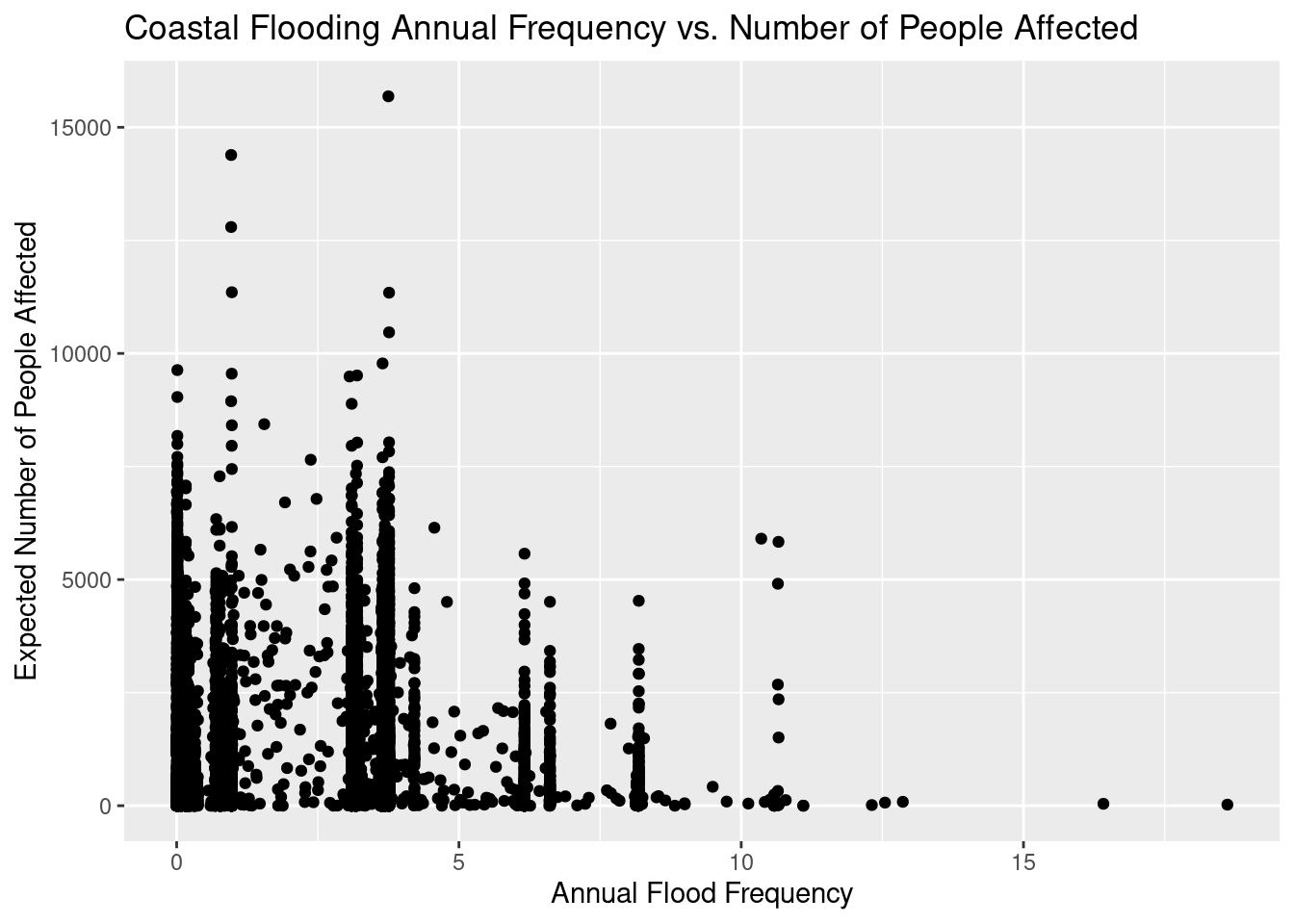
With river flooding, as seen in the last pair of plots, there are a lot of cases where either a small number of people were affected, or they were affected infrequently. It does appear to be the case that when a coastal flood occurs, it is likely to affect a lot more people than a river flooding. Given that there are a lot fewer coastal floods events than river flood events, it is interesting that the product of people affected times number of annual floods is quite similar between the two flood types.
Code
facet_labels <-c("Coastal Flooding", "Riverine Flooding")names(facet_labels) <-c("CFLD_AFREQ", "RFLD_AFREQ")df %>%select(TRACTFIPS, ends_with("AFREQ")) %>%# ends_with("EXPP")) %>% pivot_longer(!TRACTFIPS, names_to="Variable", values_to="Values") %>%filter(str_detect(Variable, "FLD")) %>%filter(!is.na(Values)) %>%filter(Values>0) %>%mutate(Variable=as.factor(Variable)) %>%ggplot(aes(x=Values)) +geom_histogram(binwidth=1) +facet_wrap(~Variable, labeller=labeller(Variable = facet_labels)) +labs(title="Annual Frequency of Flood Events By Tract",x="Number of Floods per Year",y="Number of Tracts")
Code
# Coastal Flooding vs # People affecteddf %>%filter(!is.na(CFLD_AFREQ)) %>%filter(CFLD_AFREQ>0) %>%ggplot(aes(x=CFLD_AFREQ, y=CFLD_EXPP)) +geom_point() +labs(title="Coastal Flooding Annual Frequency vs. Number of People Affected",y="Expected Number of People Affected",x="Annual Flood Frequency" )
Code
# Riverine Flooding vs # People affecteddf %>%ggplot(aes(x=RFLD_AFREQ, y=RFLD_EXPP)) +geom_point() +labs(title="Riverine Flooding Annual Frequency vs. Number of People Affected",y="Expected Number of People Affected",x="Annual Flood Frequency" )
Code
# Expected number of people affected annually (# people times # floods)facet_labels <-c("Coastal Flooding", "Riverine Flooding")names(facet_labels) <-c("CFLD", "RFLD")df %>%select(TRACTFIPS, CFLD_AFREQ, CFLD_EXPP, RFLD_AFREQ, RFLD_EXPP) %>%filter(CFLD_AFREQ+RFLD_AFREQ>0.5) %>%pivot_longer(!TRACTFIPS, names_to=c("Flood", ".value"), names_pattern="(.*FLD).*(AFREQ|EXPP)",values_drop_na =TRUE,values_to="Values") %>%mutate(Annual_effect=AFREQ*EXPP) %>%filter(Annual_effect>100) %>%ggplot(aes(x=Annual_effect)) +geom_histogram(binwidth =2000) +scale_y_log10() +# facet_wrap(~Flood) +facet_wrap(~Flood, labeller=labeller(Flood = facet_labels)) +labs(title="People times number of Floods per Year by Tract",x="People times Floods per Year",y="Number of Tracts")
Summary
This dataset has 85,154 records, representing census tracts. For each tract there are 467 variables covering 18 different disasters, with mostly economic loss numbers, but also estimates of the annual frequency and the number of people expected to be affected by that disaster.
The numbers are (I think) based on the historical records, with statistical predictions. For the Population Exposure, the numbers contained within the software package Hazus 6.0 were used. A small number of these estimates are larger than the population within the tract. I have queried the FEMA support desk, and after a week have received no reply. I assume that the people doing support have probably been DOGEd.
Source Code
---title: "Read in 2023 FEMA National Risk Estimates"author: "Alan Jackson"format: html: code-fold: true code-tools: truedescription: "Read in the FEMA National Risk Estimate table and split out by disaster"date: "4/28/2025"image: "cover.png"categories: - Mapping - Supporting Activismexecute: freeze: auto # re-render only when source changes warning: falseeditor: source---## Read in the National Risk EstimatesData downloaded from https://hazards.fema.gov/nri/data-resources#csvDownloadThis is more painful than it sounds. The csv file has 467 columns, most ofwhich are double precision, but some are character. And many are blank near thetop of the file, so automatic schemes fail. Also, the number of columns for eachdisaster type varies, so simple schemes for determining how to read the datain will fail.After (finally) getting it read in, I'll look at it and then save files by disaster.#### MetadataThe disaster codes are pretty easy to guess, but here are the definitions:| Hazard | Prefix ||:--------|:-------||Avalanche|AVLN||Coastal Flooding|CFLD||Cold Wave|CWAV||Drought|DRGT||Earthquake|ERQK||Hail| HAIL||Heat Wave|HWAV||Hurricane|HRCN||Ice Storm|ISTM||Landslide|LNDS||Lightning|LTNG||Riverine Flooding|RFLD||Strong Wind|SWND||Tornado|TRND||Tsunami|TSUN||Volcanic Activity|VLCN||Wildfire|WFIR||Winter Weather|WNTW|: {tbl-colwidths="[25,75]"}|Suffix | Meaning ||:------|:--------||EVNTS | Number of Events||AFREQ | Annualized Frequency||EXPB | Exposure - Building Value||EXPP | Exposure - Population||EXPPE | Exposure - Population Equivalence||EXPA | Exposure - Agriculture Value||EXPT | Exposure - Total||EXP_AREA | Exposure - Impacted Area (sq mi)||HLRB | Historic Loss Ratio - Buildings||HLRP | Historic Loss Ratio - Population||HLRA | Historic Loss Ratio - Agriculture||HLRR | Historic Loss Ratio - Total Rating||EALB | Expected Annual Loss - Building Value||EALP | Expected Annual Loss - Population||EALPE | Expected Annual Loss - Population Equivalence||EALA | Expected Annual Loss - Agriculture Value||EALT | Expected Annual Loss - Total||EALS | Expected Annual Loss Score||EALR | Expected Annual Loss Rating||ALRB | Expected Annual Loss Rate - Building||ALRP | Expected Annual Loss Rate - Population||ALRA | Expected Annual Loss Rate - Agriculture||ALR_NPCTL | Expected Annual Loss Rate - National Percentile||RISKV | Hazard Type Risk Index Value||RISKS | Hazard Type Risk Index Score||RISKR | Hazard Type Risk Index Rating|"Population Equivalence" is the monetary value of the exposed population, using a "value of statistical life (VSL)" approach. Each fatality or ten injuries is treated as $11.6 million of economic loss.```{r}library(tidyverse)library(sf)library(leaflet)library(gt)googlecrs <-"EPSG:4326"path <-"/home/ajackson/Dropbox/Rprojects/ERD/Data/FEMA_National_Risk_Index_Data/"Datapath <-"/home/ajackson/Dropbox/Rprojects/Curated_Data_Files/"df <-read_csv(paste0(path, "NRI_Table_CensusTracts/NRI_Table_CensusTracts.csv"))foo <-names(df)[41:466] # only look at disaster categories# are all disasters the same? No.str_sub(foo, 1, 4) %>%as_tibble() %>%count(value) %>%gt() %>%tab_header(title=md("**Count of Fields for each Disaster**") ) %>%fmt_number(columns=n,sep_mark=',',decimals=0 ) %>%cols_label(value ="Disaster Code",n ="Number of Fields" ) # Build a table to decide how to read columnCspec <-str_extract(foo, "_.*") %>%as_tibble() %>%count(value)foo2 <- foo %>%as_tibble() %>%mutate(Spec=if_else(str_detect(value, "R$"), "c", "d"))Spec <-paste0(foo2$Spec, collapse="")Col_spec=paste0(str_dup("c",11), "ddddddcddcddddddddddddcddcddd", Spec, "c")# Try againdf <-read_csv(paste0(path, "NRI_Table_CensusTracts/NRI_Table_CensusTracts.csv"),col_types = Col_spec)```### Let's check for understanding and consistencyHmmm... there are tracts where the number of people expected to be affected bythe disaster is larger than the population of the tract. ```{r}foo <- df %>%select(TRACTFIPS, POPULATION, CFLD_EXPP) %>%mutate(Pop_diff=(POPULATION - CFLD_EXPP)/POPULATION) %>%filter(Pop_diff>0) %>%filter(Pop_diff<1) %>%mutate(Pct_effected=CFLD_EXPP*100/POPULATION) ggstatsplot::gghistostats(data=foo,x=Pct_effected,xlab ="Percent of Population affected",title ="Percent of the Population in a Tract Affected by Flooding",subtitle ="After elimination of unrealistic values")df %>%select(TRACTFIPS, POPULATION, CFLD_EXPP) %>%mutate(Pop_diff=POPULATION - CFLD_EXPP) %>%filter(Pop_diff<0) %>%ggplot(aes(x=Pop_diff)) +geom_histogram() +labs(title="Population Minus Affected Population, Tracts that Flood",subtitle="For values less than zero only (bad data values?)",x="Population - Affected Population")```### Attach the polygons and make a mapTo highlight the more interesting areas, I will map only the tracts denoted by arisk rating of "very high".I'll also restrict the data to tracts with a population of greater than 100, andwith a percent of the population at flood risk greater than 25%.Not surprisingly, most of the flood risk falls near the coast.```{r}df$RISK_RATNG %>%as_tibble() %>%count(value) %>%gt() %>%tab_header(title=md("**Count of Tracts for each Risk Rating**") ) %>%fmt_number(columns=n,sep_mark=',',decimals=0 ) %>%cols_label(value ="Risk Rating",n ="Number of Tracts" )df_sub <- df %>%filter(RISK_RATNG=="Very High") %>%select(STATEABBRV, TRACTFIPS, POPULATION, RISK_VALUE, ends_with("AFREQ"), ends_with("EXPP"))# Attach tract polygonsCensus <-readRDS(paste0(Datapath, "Census_Tracts_2023/All_ACS_2023.rds"))df_sub <- df_sub %>%filter(POPULATION>100) %>%mutate(GEOID=TRACTFIPS) %>%mutate(Pop_Exposed=as.integer(pmin(100*pmax( CFLD_EXPP, RFLD_EXPP, na.rm=TRUE)/POPULATION,100))) %>%filter(Pop_Exposed>25) %>%mutate(CFLD_AFREQ=signif(CFLD_AFREQ, 3),CFLD_EXPP=as.integer(CFLD_EXPP),RFLD_AFREQ=signif(RFLD_AFREQ, 3),RFLD_EXPP=as.integer(RFLD_EXPP)) %>%inner_join(., Census, by="GEOID") %>% sf::st_as_sf()# make mappal <-colorNumeric("YlOrBr",c(min(df_sub$Pop_Exposed, na.rm=TRUE),max(df_sub$Pop_Exposed, na.rm=TRUE)),na.color ="transparent")leaflet(data=df_sub) %>%addTiles() %>%addPolygons(data=df_sub,weight=2, color="black",fillOpacity =0.4,fillColor =pal(df_sub$Pop_Exposed),popup =paste("<div class='leaflet-popup-scrolled' style='max-width:150px;max-height:200px'>","Coast Fld Ann Freq:", df_sub$CFLD_AFREQ, "<br>","Coast Fld Exp Pop:", df_sub$CFLD_EXPP, "<br>","River Fld Ann Freq:", df_sub$RFLD_AFREQ, "<br>","River Fld Exp Pop:", df_sub$RFLD_EXPP, "<br>","Total Pop:", df_sub$POPULATION, "<br>","Max % Pop Exp:", df_sub$Pop_Exposed, "</div>" )) %>%addLegend("bottomright", pal = pal, values =~df_sub$Pop_Exposed,title ="Pct Pop Exposed",opacity =1 )```### Look at FloodingWe'll look at Coastal Flooding and Riverine FloodingMany more tracts subject to river flooding, but coastal flooding has more potential to affect more people.With river flooding, as seen in the last pair of plots, there are a lot of caseswhere either a small number of people were affected, or they were affectedinfrequently. It does appear to be the case that when a coastal flood occurs, itis likely to affect a lot more people than a river flooding. Given that there are a lot fewer coastal floods events than river flood events, it is interesting that the product of people affected times number of annual floods is quite similar between the two flood types.```{r}facet_labels <-c("Coastal Flooding", "Riverine Flooding")names(facet_labels) <-c("CFLD_AFREQ", "RFLD_AFREQ")df %>%select(TRACTFIPS, ends_with("AFREQ")) %>%# ends_with("EXPP")) %>% pivot_longer(!TRACTFIPS, names_to="Variable", values_to="Values") %>%filter(str_detect(Variable, "FLD")) %>%filter(!is.na(Values)) %>%filter(Values>0) %>%mutate(Variable=as.factor(Variable)) %>%ggplot(aes(x=Values)) +geom_histogram(binwidth=1) +facet_wrap(~Variable, labeller=labeller(Variable = facet_labels)) +labs(title="Annual Frequency of Flood Events By Tract",x="Number of Floods per Year",y="Number of Tracts")# Coastal Flooding vs # People affecteddf %>%filter(!is.na(CFLD_AFREQ)) %>%filter(CFLD_AFREQ>0) %>%ggplot(aes(x=CFLD_AFREQ, y=CFLD_EXPP)) +geom_point() +labs(title="Coastal Flooding Annual Frequency vs. Number of People Affected",y="Expected Number of People Affected",x="Annual Flood Frequency" )# Riverine Flooding vs # People affecteddf %>%ggplot(aes(x=RFLD_AFREQ, y=RFLD_EXPP)) +geom_point() +labs(title="Riverine Flooding Annual Frequency vs. Number of People Affected",y="Expected Number of People Affected",x="Annual Flood Frequency" )# Expected number of people affected annually (# people times # floods)facet_labels <-c("Coastal Flooding", "Riverine Flooding")names(facet_labels) <-c("CFLD", "RFLD")df %>%select(TRACTFIPS, CFLD_AFREQ, CFLD_EXPP, RFLD_AFREQ, RFLD_EXPP) %>%filter(CFLD_AFREQ+RFLD_AFREQ>0.5) %>%pivot_longer(!TRACTFIPS, names_to=c("Flood", ".value"), names_pattern="(.*FLD).*(AFREQ|EXPP)",values_drop_na =TRUE,values_to="Values") %>%mutate(Annual_effect=AFREQ*EXPP) %>%filter(Annual_effect>100) %>%ggplot(aes(x=Annual_effect)) +geom_histogram(binwidth =2000) +scale_y_log10() +# facet_wrap(~Flood) +facet_wrap(~Flood, labeller=labeller(Flood = facet_labels)) +labs(title="People times number of Floods per Year by Tract",x="People times Floods per Year",y="Number of Tracts")```### SummaryThis dataset has 85,154 records, representing census tracts. For each tractthere are 467 variables covering 18 different disasters, with mostly economicloss numbers, but also estimates of the annual frequency and the number ofpeople expected to be affected by that disaster.The numbers are (I think) based on the historical records, with statistical predictions. For the Population Exposure, the numbers contained within thesoftware package Hazus 6.0 were used. A small number of these estimates arelarger than the population within the tract. I have queried the FEMA support desk, and after a week have received no reply. I assume that the people doingsupport have probably been DOGEd.