Create rasters by census tract with sea level rise and dasymetric data in them.
Author
Alan Jackson
Published
June 15, 2025
Sea level rise and population distribution
For each census tract, create a series of sea level rise grids for 0-10 feet of sea level rise. On the same grid coordinates, cut the dasymetric grid for the lower 48.
The grids will be saved at 90 meter grid spacing, converted to WGS84 and lat-long coordinates. The water depths will be in feet. Population estimates for a grid cell less than 0.1 person will be set to NA.
Sea level rise data comes from https://coast.noaa.gov/slrdata/Depth_Rasters/index.html
To download the files, a convenient file of URL’s is supplied: wget –input-file=URLlist_SC.txt
Dasymetric grid comes from https://catalog.data.gov/dataset/enviroatlas-2020-dasymetric-population-for-the-conterminous-united-states-v1-12
Tract boundaries come from the 2020 census data via tidycensus.
Process outline
Minimize coordinate projections
Attach dasym
Get tracts for a state
project tracts to googlecrs
read in a tile
resample tile to 30 m (factor=9)
project tile to googlecrs
for each SL tile, find intersecting tracts
get extent of SL tile
project extent to Albers
cut out dasym
project cutout to googlecrs and resample to tile grid
cut SL tile for each intersecting tract and save
cut dasym tile by tract and save
Testing stub
Code
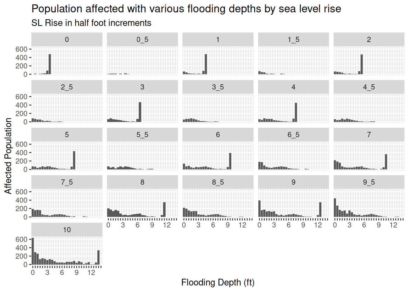
# #| eval: false#| warning: false#| echo: false#| message: false############################### Attach dasymetric file and get the geodetics for it##############################State <-"LA"file <-"2020_Dasymetric_Population_CONUS_V1_1.tif"x <- terra::rast(paste0(Dasym_path, "2020_Dasymetric_Population_CONUS_V1_1.tif")) ############################### - read in a tile and resample############################### Read in tile and change grid spacing to 30 m from 10 mSL_orig <- terra::aggregate( terra::rast(paste0(SL_path, "LA_CentralEast_slr_depth_3ft.tif")), fact=3, fun="median", na.rm=TRUE)# Get rid of flagsSL_orig <- terra::ifel(SL_orig >9, NA, SL_orig)# convert depths to feetSL_orig <- SL_orig*3.28084############################### Project dasym file onto SL coordinates##############################Dasym <- terra::project(x, SL_orig, method="sum")############################### Make a 2-layer file and save##############################Combo <-c(Dasym, SL_orig) %>% tidyterra::rename(Pop='2020_Dasymetric_Population_CONUS_V1_1',Depth='LA_CentralEast_slr_depth_3ft') # terra::writeRaster(Combo, paste0(Combo_path, file), overwrite=TRUE)############################### - Get tracts for a state and convert to NAD83##############################Tracts <-readRDS(paste0(Census_path, "ACS_2023_", State, ".rds"))Tracts <- Tracts %>% sf::st_transform(crs=terra::crs(Dasym)) %>%filter(!sf::st_is_empty(.)) %>%# remove empty collections sf::st_make_valid()# Make some plots# tmap::tmap_options(basemaps="OpenStreetMap")tmap_options(basemap.server =c("OpenStreetMap"))tmap_mode <- tmap::tmap_mode("view") # set mode to interactive plotstmap::tm_shape(terra::ifel(Dasym >10, 10, Dasym)) + tmap::tm_raster(col_alpha=0.7,# palette = "brewer.reds",col.scale =tm_scale(values="brewer.reds"),col.legend =tm_legend(title="Dasym") )
Code
# title = "Dasym")tmap::tm_shape(terra::as.polygons(terra::ext(Combo))) + tmap::tm_polygons(fill_alpha=0.0, col="blue", lwd=3)
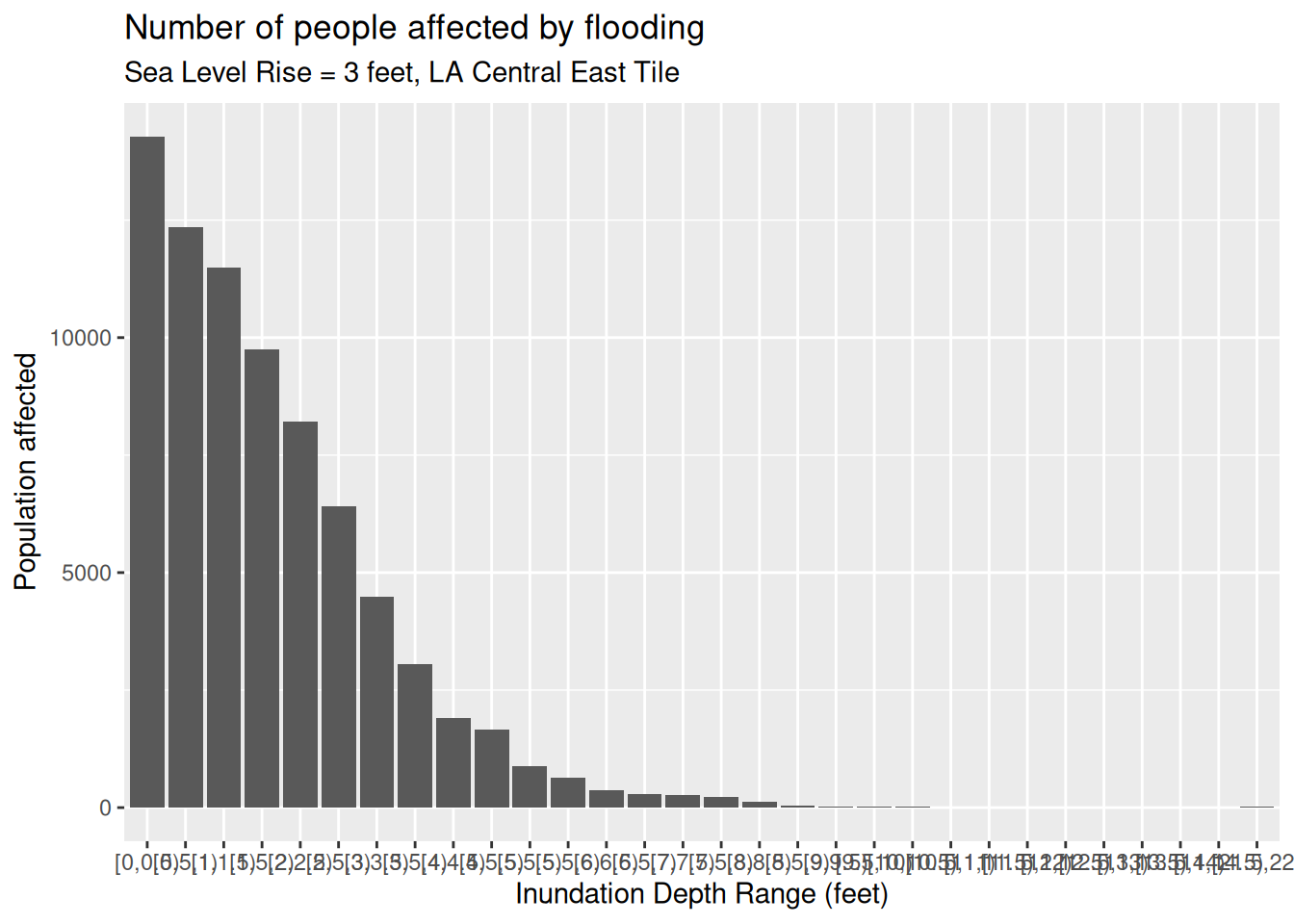
# title = "SL_orig")############################### - for each SL tile, find intersecting tracts############################### Pull out only tracts that intersect the spatrasterterra::gdalCache(size =2000)foo <- prioritizr::intersecting_units(Tracts, SL_orig)Tract_trim <- Tracts[foo,]############################### - For each tract, calculate statistics##############################val_by_tract <- exactextractr::exact_extract(progress=FALSE,x=Combo,y=Tract_trim,include_cols=c("GEOID","PopE")) %>% dplyr::bind_rows() %>% tibble::as_tibble()Values_by_node <- val_by_tract %>%filter(Pop>0) %>%# drop nodes with zero populationreplace_na(list(Depth=-1)) %>%mutate(Depth_bins=cut_width(Depth, width=0.5, center=0.25, closed="left")) Stats_by_tract <- Values_by_node %>%group_by(GEOID, Depth_bins) %>%summarize(PopE=first(PopE),Pop=sum(Pop*coverage_fraction),Num=sum(coverage_fraction) )############################### Stats for entire tile, and plot##############################Tract_pops <- Stats_by_tract %>%group_by(GEOID) %>%summarise(Pop_tot=sum(Pop),Area_tot=sum(Num) ) %>%ungroup()Stats_by_tract <- Stats_by_tract %>%left_join(., Tract_pops, by="GEOID") %>%mutate(Pop_pct=Pop/Pop_tot,Area_pct=Num/Area_tot) %>%ungroup()Stats_by_tract2 <- Stats_by_tract %>%filter(Pop>=1) %>%filter(Depth_bins!="[-1,-0.5)") %>%group_by(Depth_bins) %>%summarise(Affected=sum(Pop) ) %>%ungroup()Stats_by_tract2 %>%ggplot(aes(x=Depth_bins, y=Affected)) +geom_bar(stat="identity") +labs(title="Number of people affected by flooding",subtitle="Sea Level Rise = 3 feet, LA Central East Tile",x="Inundation Depth Range (feet)",y="Population affected")
Let’s do Louisiana
First let’s look at the tile extents
It appears that they must overlap a great deal, since the actual data appears to follow parish/county boundaries. But let’s make sure that is the case.
The tile extents are defined by the county lines, so much of the area around the edges of the tiles is set to NA, so we must work with only the tracts entirely contained within the tile extents, to avoid getting bogus results.
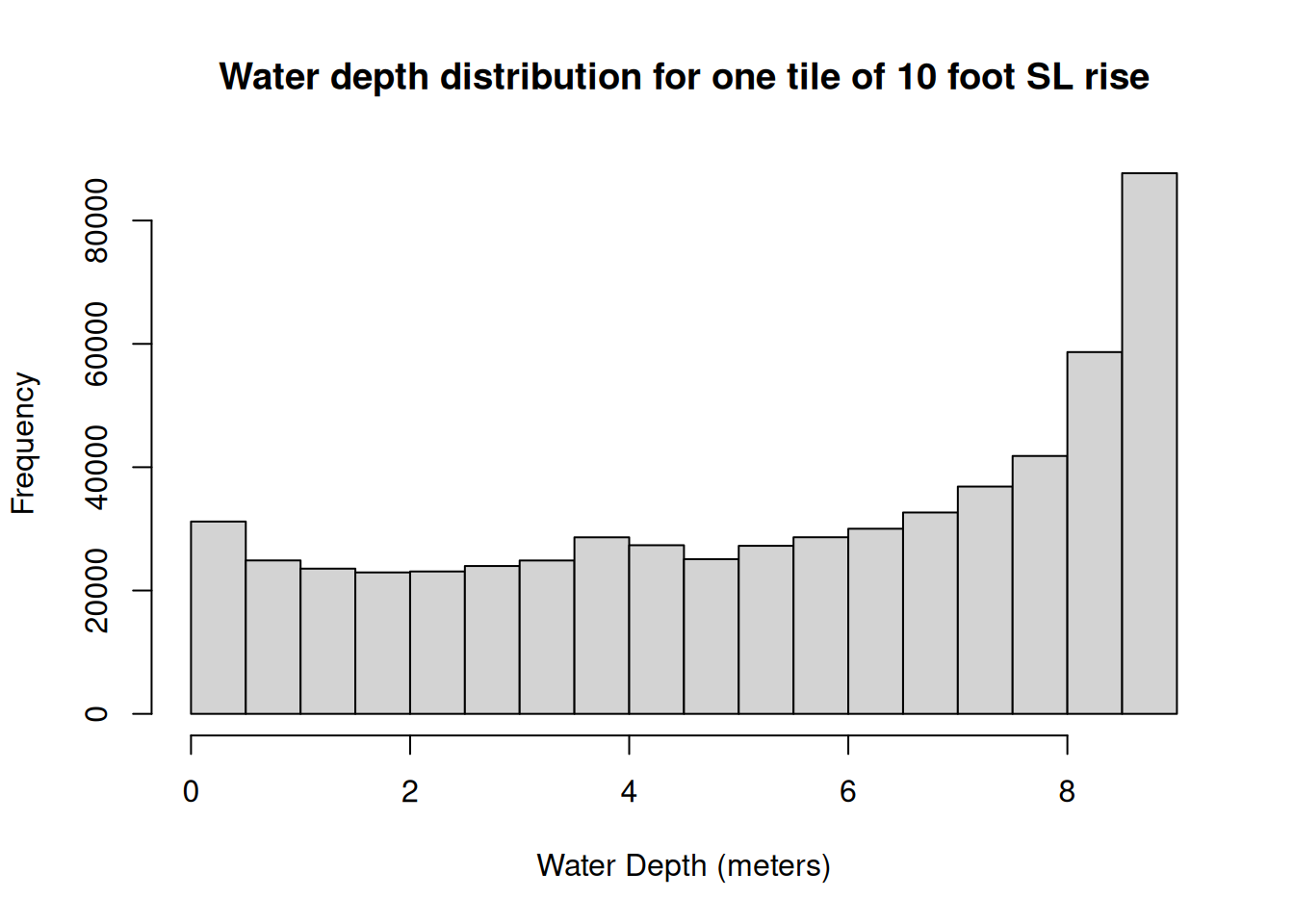
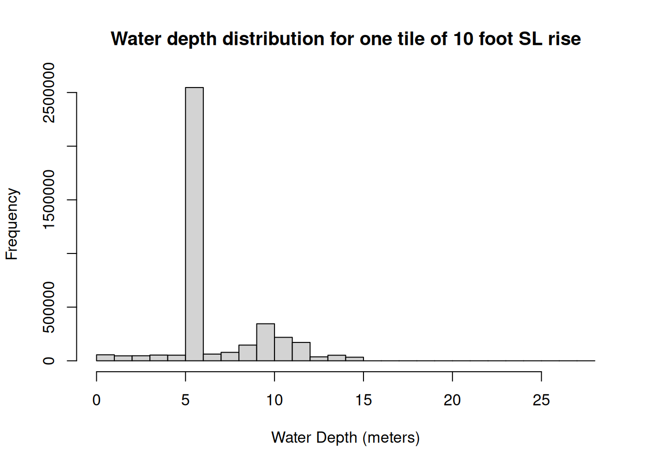
For the map, I set the NA values equal to 6, so that they will appear on the map. The values in the sea level grid are meters of water depth, with values greater than 9 representing current water surfaces.
Thankfully, the map shows that the tiles were designed very well, such that when tile boundaries cut tract boundaries, the grid nodes within the partial tract are set to null.
Code
# #| eval: false #| warning: false#| echo: false#| message: false# Modified to use resampled tilesState <-"LA"infiles <-list.files(path=Combo_path, pattern=paste0("^",State,"_.*\\.tif$")) infiles <- infiles[stringr::str_detect(infiles, "Depth")]Basenames <- infiles %>% stringr::str_remove(., "_Depth_.*tif") %>%unique()Depth_names <-as.character(0:20/2) %>% stringr::str_remove(., "\\.0$") %>% stringr::str_replace(., "\\.", "_")SL <-Depth_names[21] i <-1for (Tilename in Basenames){ memories <-gc()# Read in tile SL_temp <- terra::rast(paste0(Combo_path, Tilename, "_Depth_",SL ,".tif")) if (i==1) { Extents <- terra::as.polygons(terra::ext(SL_temp), crs=terra::crs(SL_temp)) } else { Extents <-rbind(Extents, terra::as.polygons(terra::ext(SL_temp),crs=terra::crs(SL_temp))) } i <- i +1}memories <-gc() # free memorySL_temp <- terra::aggregate( terra::rast(paste0(Combo_path, Basenames[1], "_Depth_",SL ,".tif")), fact=3, fun="median", na.rm=TRUE)SL_water <- terra::ifel(SL_temp >9, NA, SL_temp)SL_temp <- terra::ifel(is.nan(SL_temp), 6, SL_temp)hist(SL_water[!is.na(SL_water)], xlab="Water Depth (meters)",main="Water depth distribution for one tile of 10 foot SL rise")
Code
hist(SL_temp[!is.na(SL_temp)], xlab="Water Depth (meters)",main="Water depth distribution for one tile of 10 foot SL rise")
First lets resample the dasym file once and save it so we don’t pay that expense more than once.
Code
# Resample the dasymmetric file and save itx <- terra::rast(paste0(Dasym_path, "2020_Dasymetric_Population_CONUS_V1_1.tif")) print("Read in dasym and resample")# Change grid spacing to 90 m from 30 mx <- terra::aggregate(x, fact=3, fun="sum", na.rm=TRUE)# Save resampled fileterra::writeRaster(x, paste0(Dasym_path, "2020_Dasymetric_Population_CONUS_V1_1_resamp90m.tif"),overwrite=TRUE)
For each state, save resampled tiles and a tract by tract summary
Especially for California, there is a lot of cruft to deal with. Some tiles have no water, the extents may not be consistent, so those cases must be dealt with.
Some of the California files have different extents, so we needed to test ways to deal with that. Also, two files (as shown below) were in projected coordinates instead of geographic, so we had to project them into geographic coordinates in order for the process to proceed.
Some of the Virginia are projected to XY coordinates instead of geographic, so we had to project them into geographic coordinates in order for the process to proceed. The Mid and N files in particular.
Code
State="VA"files <-list.files(path=SL_path, pattern=paste0("^",State,"_N.*ft\\.tif$"))Template <- terra::rast(paste0(SL_path, files[1]))############## fix rasters that were projected to XYfor (file in files) { Old_rast <- terra::rast(paste0(SL_path, file)) footest <- stringr::str_extract(terra::crs(Old_rast), "^.*\\[")print(paste(file, footest))if (footest=="GEOGCRS[") {next } else { New_rast <- terra::project(Old_rast, terra::crs(Template)) terra::writeRaster(New_rast, paste0(SL_path, file),overwrite=TRUE) }}
Check states for redo
Ugh. They all need to be redone to fix depth bins.
---title: "Build Sea Level Rise census Tracts and Dasymetric Tracts"author: "Alan Jackson"format: html: code-fold: true code-tools: truedescription: "Create rasters by census tract with sea level rise and dasymetric data in them."date: "6/15/2025"image: "cover.png"categories: - Census - Episcopal Relief and Development - Sea Level - Mapping - Supporting Activismexecute: freeze: auto # re-render only when source changes warning: falseeditor: source---## Sea level rise and population distributionFor each census tract, create a series of sea level rise grids for 0-10 feetof sea level rise. On the same grid coordinates, cut the dasymetric grid forthe lower 48.The grids will be saved at 90 meter grid spacing, converted to WGS84 andlat-long coordinates. The water depths will be in feet. Population estimatesfor a grid cell less than 0.1 person will be set to NA.Sea level rise data comes from https://coast.noaa.gov/slrdata/Depth_Rasters/index.htmlTo download the files, a convenient file of URL's is supplied:wget --input-file=URLlist_SC.txtDasymetric grid comes from https://catalog.data.gov/dataset/enviroatlas-2020-dasymetric-population-for-the-conterminous-united-states-v1-12Tract boundaries come from the 2020 census data via tidycensus.```{r}#| warning: false#| echo: false#| message: falselibrary(tidyverse)library(terra)library(tidyterra)library(sf)library(tmap)terra::terraOptions(progress =0)options(dplyr.summarise.inform =FALSE)tmap::tmap_options(show.messages=FALSE, show.warnings=FALSE)# SL_path <- "/home/ajackson/Sea_Level_Temp/"SL_path <-"/media/ajackson/extradrive1/original_sealevel/"Dasym_path <-"/home/ajackson/Dropbox/Rprojects/Curated_Data_Files/Dasymetric/2020_Dasymetric_Population_CONUS_V1_1/"Census_path <-"/home/ajackson/Dropbox/Rprojects/Curated_Data_Files/Census_Tracts_2023/"Combo_path <-"/home/ajackson/Dropbox/Rprojects/Curated_Data_Files/Dasym_SL_Combos/"path <-"/home/ajackson/Dropbox/Rprojects/Curated_Data_Files/SL_Dasym_Tracts/"Census_crs <-"EPSG:4269"Google_crs <-"EPSG:4326"SL_crs <-"EPSG:4269"```### Process outline- Minimize coordinate projections- Attach dasym- Get tracts for a state- project tracts to googlecrs- read in a tile- resample tile to 30 m (factor=9)- project tile to googlecrs- for each SL tile, find intersecting tracts - get extent of SL tile - project extent to Albers - cut out dasym - project cutout to googlecrs and resample to tile grid - cut SL tile for each intersecting tract and save - cut dasym tile by tract and save### Testing stub```{r}# #| eval: false#| warning: false#| echo: false#| message: false############################### Attach dasymetric file and get the geodetics for it##############################State <-"LA"file <-"2020_Dasymetric_Population_CONUS_V1_1.tif"x <- terra::rast(paste0(Dasym_path, "2020_Dasymetric_Population_CONUS_V1_1.tif")) ############################### - read in a tile and resample############################### Read in tile and change grid spacing to 30 m from 10 mSL_orig <- terra::aggregate( terra::rast(paste0(SL_path, "LA_CentralEast_slr_depth_3ft.tif")), fact=3, fun="median", na.rm=TRUE)# Get rid of flagsSL_orig <- terra::ifel(SL_orig >9, NA, SL_orig)# convert depths to feetSL_orig <- SL_orig*3.28084############################### Project dasym file onto SL coordinates##############################Dasym <- terra::project(x, SL_orig, method="sum")############################### Make a 2-layer file and save##############################Combo <-c(Dasym, SL_orig) %>% tidyterra::rename(Pop='2020_Dasymetric_Population_CONUS_V1_1',Depth='LA_CentralEast_slr_depth_3ft') # terra::writeRaster(Combo, paste0(Combo_path, file), overwrite=TRUE)############################### - Get tracts for a state and convert to NAD83##############################Tracts <-readRDS(paste0(Census_path, "ACS_2023_", State, ".rds"))Tracts <- Tracts %>% sf::st_transform(crs=terra::crs(Dasym)) %>%filter(!sf::st_is_empty(.)) %>%# remove empty collections sf::st_make_valid()# Make some plots# tmap::tmap_options(basemaps="OpenStreetMap")tmap_options(basemap.server =c("OpenStreetMap"))tmap_mode <- tmap::tmap_mode("view") # set mode to interactive plotstmap::tm_shape(terra::ifel(Dasym >10, 10, Dasym)) + tmap::tm_raster(col_alpha=0.7,# palette = "brewer.reds",col.scale =tm_scale(values="brewer.reds"),col.legend =tm_legend(title="Dasym") )# title = "Dasym")tmap::tm_shape(terra::as.polygons(terra::ext(Combo))) + tmap::tm_polygons(fill_alpha=0.0, col="blue", lwd=3) tmap::tm_shape(SL_orig) + tmap::tm_raster(col_alpha=0.7,# palette = "brewer.blues",col.scale =tm_scale(values="brewer.blues"),col.legend =tm_legend(title="SL_orig") )# title = "SL_orig")############################### - for each SL tile, find intersecting tracts############################### Pull out only tracts that intersect the spatrasterterra::gdalCache(size =2000)foo <- prioritizr::intersecting_units(Tracts, SL_orig)Tract_trim <- Tracts[foo,]############################### - For each tract, calculate statistics##############################val_by_tract <- exactextractr::exact_extract(progress=FALSE,x=Combo,y=Tract_trim,include_cols=c("GEOID","PopE")) %>% dplyr::bind_rows() %>% tibble::as_tibble()Values_by_node <- val_by_tract %>%filter(Pop>0) %>%# drop nodes with zero populationreplace_na(list(Depth=-1)) %>%mutate(Depth_bins=cut_width(Depth, width=0.5, center=0.25, closed="left")) Stats_by_tract <- Values_by_node %>%group_by(GEOID, Depth_bins) %>%summarize(PopE=first(PopE),Pop=sum(Pop*coverage_fraction),Num=sum(coverage_fraction) )############################### Stats for entire tile, and plot##############################Tract_pops <- Stats_by_tract %>%group_by(GEOID) %>%summarise(Pop_tot=sum(Pop),Area_tot=sum(Num) ) %>%ungroup()Stats_by_tract <- Stats_by_tract %>%left_join(., Tract_pops, by="GEOID") %>%mutate(Pop_pct=Pop/Pop_tot,Area_pct=Num/Area_tot) %>%ungroup()Stats_by_tract2 <- Stats_by_tract %>%filter(Pop>=1) %>%filter(Depth_bins!="[-1,-0.5)") %>%group_by(Depth_bins) %>%summarise(Affected=sum(Pop) ) %>%ungroup()Stats_by_tract2 %>%ggplot(aes(x=Depth_bins, y=Affected)) +geom_bar(stat="identity") +labs(title="Number of people affected by flooding",subtitle="Sea Level Rise = 3 feet, LA Central East Tile",x="Inundation Depth Range (feet)",y="Population affected")```### Let's do Louisiana### First let's look at the tile extentsIt appears that they must overlap a great deal, since the actual data appears tofollow parish/county boundaries. But let's make sure that is the case.The tile extents are defined by the county lines, so much of the area around the edges of the tiles is set to NA, so we must work with only the tractsentirely contained within the tile extents, to avoid getting bogus results.For the map, I set the NA values equal to 6, so that they will appear on themap. The values in the sea level grid are meters of water depth, withvalues greater than 9 representing current water surfaces.Thankfully, the map shows that the tiles were designed very well, such that whentile boundaries cut tract boundaries, the grid nodes within the partial tractare set to null.```{r}# #| eval: false #| warning: false#| echo: false#| message: false# Modified to use resampled tilesState <-"LA"infiles <-list.files(path=Combo_path, pattern=paste0("^",State,"_.*\\.tif$")) infiles <- infiles[stringr::str_detect(infiles, "Depth")]Basenames <- infiles %>% stringr::str_remove(., "_Depth_.*tif") %>%unique()Depth_names <-as.character(0:20/2) %>% stringr::str_remove(., "\\.0$") %>% stringr::str_replace(., "\\.", "_")SL <-Depth_names[21] i <-1for (Tilename in Basenames){ memories <-gc()# Read in tile SL_temp <- terra::rast(paste0(Combo_path, Tilename, "_Depth_",SL ,".tif")) if (i==1) { Extents <- terra::as.polygons(terra::ext(SL_temp), crs=terra::crs(SL_temp)) } else { Extents <-rbind(Extents, terra::as.polygons(terra::ext(SL_temp),crs=terra::crs(SL_temp))) } i <- i +1}memories <-gc() # free memorySL_temp <- terra::aggregate( terra::rast(paste0(Combo_path, Basenames[1], "_Depth_",SL ,".tif")), fact=3, fun="median", na.rm=TRUE)SL_water <- terra::ifel(SL_temp >9, NA, SL_temp)SL_temp <- terra::ifel(is.nan(SL_temp), 6, SL_temp)hist(SL_water[!is.na(SL_water)], xlab="Water Depth (meters)",main="Water depth distribution for one tile of 10 foot SL rise")hist(SL_temp[!is.na(SL_temp)], xlab="Water Depth (meters)",main="Water depth distribution for one tile of 10 foot SL rise")# Get tracts *contained* within tile extentTracts <-readRDS(paste0(Census_path, "ACS_2023_", State, ".rds"))Extent <- sf::st_as_sf(terra::as.polygons(terra::ext(SL_temp), crs=terra::crs(SL_temp)))Extent <- sf::st_transform(Extent, crs=sf::st_crs(Tracts))foobar <- sf::st_within(Tracts, Extent, sparse=FALSE)Tract_trim <- Tracts[foobar,]tmap::tmap_options(basemap.server =c("OpenStreetMap"))tmap::tmap_mode("view") # set mode to interactive plotstmap::tm_shape(Extents) + tmap::tm_polygons(fill_alpha=0.0, col="blue", lwd=3)+tmap::tm_shape(SL_temp) + tmap::tm_raster(col_alpha=0.7,col.scale =tm_scale(values="brewer.blues"),col.legend =tm_legend(title="Inches Flooding") ) +# palette = "brewer.blues",# title = "Inches flooding") +tmap::tm_shape(Tracts) + tmap::tm_polygons(fill_alpha=0.0, col="pink", lwd=1) +tmap::tm_shape(Tract_trim) + tmap::tm_polygons(fill_alpha=0.0, col="red", lwd=3) ```### And here we do the real workFirst lets resample the dasym file *once* and save it so we don't pay that expense more than once.```{r}#| eval: false# Resample the dasymmetric file and save itx <- terra::rast(paste0(Dasym_path, "2020_Dasymetric_Population_CONUS_V1_1.tif")) print("Read in dasym and resample")# Change grid spacing to 90 m from 30 mx <- terra::aggregate(x, fact=3, fun="sum", na.rm=TRUE)# Save resampled fileterra::writeRaster(x, paste0(Dasym_path, "2020_Dasymetric_Population_CONUS_V1_1_resamp90m.tif"),overwrite=TRUE)```### Function to get max extent from a set of tiles```{r}max_extent <-function(files, path) {# files <- list.files(path=SL_path, pattern=paste0("^",State,"_EKA_.*ft\\.tif$")) Tile_xmin <-0 Tile_xmax <-0 Tile_ymin <-0 Tile_ymax <-0for (file in files) { Xtnt <- terra::ext(terra::rast(paste0(path, file)))# print(paste0(path, file)) Tile_xmin <-min(Tile_xmin, Xtnt$xmin) Tile_xmax <-min(Tile_xmax, Xtnt$xmax) Tile_ymin <-max(Tile_ymin, Xtnt$ymin) Tile_ymax <-max(Tile_ymax, Xtnt$ymax)# print(paste(Tile_xmin, Tile_xmax, Tile_ymin, Tile_ymax)) }return(terra::ext(c(Tile_xmin, Tile_xmax, Tile_ymin, Tile_ymax)))}```### For each state, save resampled tiles and a tract by tract summaryEspecially for California, there is a lot of cruft to deal with.Some tiles have no water, the extents may not be consistent, so those casesmust be dealt with.```{r}#| warning: false#| echo: false#| message: falseState <-"DC"Depth_names <-as.character(0:20/2) %>% stringr::str_remove(., "\\.0$") %>% stringr::str_replace(., "\\.", "_")############################### Attach dasymetric file and get the geodetics for it############################### print("Read in dasym")x <- terra::rast(paste0(Dasym_path, "2020_Dasymetric_Population_CONUS_V1_1_resamp90m.tif"))############################### Get tile basenames for state##############################infiles <-list.files(path=SL_path, pattern=paste0("^",State,"_.*ft\\.tif$")) Basenames <- infiles %>% stringr::str_remove(., "_slr_depth_.*tif") %>%unique()############################### - Get tracts for a state ##############################Tracts <-readRDS(paste0(Census_path, "ACS_2023_", State, ".rds"))memories <-gc() # free memory############################### Loop through basenames##############################for (Tilename in Basenames){# Tilename <- Basenames[1]print("==============================")print(paste("Tilename =", Tilename))print("==============================")############################### Data frame for accumulating values############################## All_Stats_by_tract <-NULL############################### Loop through SL depths##############################for (SL in Depth_names) {# print(paste("SL =", SL)) memories <-gc() # Free memory############################### Read in a tile and resample & clean up############################### Test filename, and update if file is badly named SL_file <- SLif (!file.exists(paste0(SL_path, Tilename, "_slr_depth_",SL ,"ft.tif"))) { SL_file <-paste0(SL, "_0") }# Still not there. Some Calif tiles lack 0.5 foot incrementsif (!file.exists(paste0(SL_path, Tilename, "_slr_depth_",SL_file ,"ft.tif"))) {# print("Skip")next# skip to next depth iteration }# print("Read in a tile and resample & clean up")# Read in tile and change grid spacing to 90 m from 10 m SL_orig <- terra::aggregate( terra::rast(paste0(SL_path, Tilename, "_slr_depth_",SL_file ,"ft.tif")), fact=9, fun="median", na.rm=TRUE)# Get rid of flags SL_orig <- terra::ifel(SL_orig >9, NA, SL_orig)# convert depths to feet SL_orig <- SL_orig*3.28084if (SL !="0") {# if tile is shorter than it should be, add nan's to puff it up. SL_orig <- terra::extend(SL_orig, Max_extent)if (terra::ext(SL_orig) != terra::ext(Dasym)) { SL_orig <- terra::project(SL_orig, Dasym) }# print("+++++++++++++++++++++++++++++++++++++++")# print(paste("Extent of", SL, terra::ext(SL_orig)))# print("+++++++++++++++++++++++++++++++++++++++") }############################### Project dasym file onto SL coordinates first time through only# Also project Tract file##############################if (SL =="0") { # print("SL==0")# Get maximum extent files <-list.files(path=SL_path, pattern=paste0("^",Tilename,"_.*ft\\.tif$")) Max_extent <-max_extent(files, SL_path)# print(paste("Max extent", Max_extent))# Enlarge base tile SL_orig <- terra::extend(SL_orig, Max_extent) Dasym <- terra::project(x, SL_orig, method="sum") %>%# sum pops when projecting tidyterra::rename(Pop='2020_Dasymetric_Population_CONUS_V1_1')# Save this Dasym grid terra::writeRaster(Dasym, paste0(Combo_path, Tilename,"_Dasym.tif"),overwrite=TRUE) Tracts <- Tracts %>% sf::st_transform(crs=terra::crs(Dasym)) %>%filter(!sf::st_is_empty(.)) %>%# remove empty collections sf::st_make_valid() %>%mutate(Real_area=units::drop_units(sf::st_area(.)))# Get tracts *contained* within tile extent Extent <- sf::st_as_sf(terra::as.polygons(terra::ext(SL_orig), crs=terra::crs(SL_orig))) Extent <- sf::st_transform(Extent, crs=sf::st_crs(Tracts)) foo <- sf::st_within(Tracts, Extent, sparse=FALSE) Tract_trim <- Tracts[foo,] }############################### save processed file############################### print("save processed file")# print(paste("Layer names:", names(SL_orig))) memories <-gc() # free memory# Get sizes of all objects in the workspace object_sizes <-sapply(ls(), function(x) object.size(get(x)))# Sort the sizes in descending order sorted_sizes <-sort(object_sizes, decreasing =TRUE)# Display the top 5 largest objects# print(head(sorted_sizes, 5))# print("rename") New_depth <-paste0("Depth_", SL) SL_orig <- SL_orig %>% tidyterra::rename(!!New_depth :=names(SL_orig)) memories <-gc() # free memory terra::writeRaster(SL_orig, paste0(Combo_path, Tilename,"_", New_depth,".tif"),overwrite=TRUE) memories <-gc() # free memory############################### - For each tract, calculate statistics############################### print("For each tract, calculate statistics")# print("val_by_tract") val_by_tract <- exactextractr::exact_extract(progress=FALSE,x=c(Dasym, SL_orig),y=Tract_trim,include_cols=c("GEOID","PopE", "Real_area")) %>% dplyr::bind_rows() %>% tibble::as_tibble()# print("Values_by_bin") Values_by_bin <- val_by_tract %>%filter(Pop>0) %>%# drop nodes with zero populationmutate(!!sym(New_depth) :=replace_na(!!sym(New_depth), -1)) # finesse case where all values are -1 for water depthif (Values_by_bin[1,5]==-1) {Values_by_bin[1,5] <-0} Values_by_bin <- Values_by_bin %>%mutate(Depth_bins=cut_width(!!sym(New_depth), width=0.5, center=0.25, closed="left")) %>%mutate(Depth_bins=stringr::str_replace(Depth_bins, "]", ")")) # fix depth bins# rm(val_by_tract) memories <-gc() # Free memory# print("Stats_by_tract") Stats_by_tract <- Values_by_bin %>%group_by(GEOID, Depth_bins) %>%summarize(PopE=first(PopE),Pop=sum(Pop*coverage_fraction),Real_area=first(Real_area),Num=sum(coverage_fraction) ) %>%ungroup() %>%mutate(SL_depth=SL)# rm(Values_by_bin) Tract_pops <- Stats_by_tract %>%# Sum up population and areagroup_by(GEOID) %>%summarise(Pop_tot=sum(Pop),Area_tot=sum(Num) ) %>%ungroup()# print("Stats_by_tract again") Stats_by_tract <- Stats_by_tract %>%# attach pop sum and calc per capitaleft_join(., Tract_pops, by="GEOID") %>%mutate(Pop_pct=Pop/Pop_tot,Area_pct=Num/Area_tot) %>%ungroup() %>%mutate(Pop=round(Pop),Pop_tot=round(Pop_tot),Pop_pct=round(Pop_pct, 2),Area_pct=round(Area_pct, 3),Area_ratio=Area_tot/Real_area )# print("All_Stats_by_tract") All_Stats_by_tract <-rbind(All_Stats_by_tract, Stats_by_tract) }write_rds(All_Stats_by_tract, paste0(Combo_path, paste0(Tilename,".rds"))) memories <-gc() # free memory}All_levels <-levels(as_factor(unique(All_Stats_by_tract$Depth_bins)))Last_level <- All_levels[length(All_levels)]Last_level <-as.numeric(stringr::str_extract(Last_level, "\\d+"))Skip <-as.integer(Last_level/5+.5)Depth_labels <-seq(0, Last_level, Skip)New_depth_labs <-NULLfor (i in Depth_labels) { New_depth_labs <-c(New_depth_labs, as.character(i), rep("", 2*Skip-1))}# New_depth_labs <- c(New_depth_labs, )All_Stats_by_tract <- All_Stats_by_tract %>%arrange(as.numeric(stringr::str_extract(Depth_bins, "\\d+")))All_Stats_by_tract$factorbins <-as_factor(All_Stats_by_tract$Depth_bins)All_Stats_by_tract %>%filter(Depth_bins!="[-1,-0.5)") %>%ggplot(aes(x=factorbins)) +geom_histogram(stat="count") +coord_flip() All_Stats_by_tract %>%filter(Depth_bins!="[-1,-0.5)") %>%mutate(SL_depth=as_factor(SL_depth)) %>%ggplot(aes(x=factorbins, y=Pop)) +geom_bar(stat="identity") +facet_wrap(~SL_depth) +scale_x_discrete(labels = New_depth_labs) +labs(title="Population affected with various flooding depths by sea level rise",subtitle="SL Rise in half foot increments",y="Affected Population",x="Flooding Depth (ft)")```### Fix CA filesSome of the California files have different extents, so we needed to test waysto deal with that. Also, two files (as shown below) were in projectedcoordinates instead of geographic, so we had to project them into geographiccoordinates in order for the process to proceed.```{r}#| eval: falseState="CA"files <-list.files(path=SL_path, pattern=paste0("^",State,"_MTR23_.*ft\\.tif$"))Tile_xmax <-NULLTile_ymin <-NULLTile_ymax <-NULLfor (file in files) {print(file)print(terra::ext(terra::rast(paste0(SL_path, file)))) Xtnt <- terra::ext(terra::rast(paste0(SL_path, file))) Tile_xmin <-min(Tile_xmin, Xtnt$xmin) Tile_xmax <-min(Tile_xmax, Xtnt$xmax) Tile_ymin <-max(Tile_ymin, Xtnt$ymin) Tile_ymax <-max(Tile_ymax, Xtnt$ymax)}Max_size <- terra::ext(c(Tile_xmin, Tile_xmax, Tile_ymin, Tile_ymax))############## fix rasters that were projected to XYTemplate <- terra::rast(paste0(SL_path, files[6]))Old_rast <- terra::rast(paste0(SL_path, files[7]))New_rast <- terra::project(Old_rast, terra::crs(Template))terra::writeRaster(New_rast, paste0(SL_path, files[7]),overwrite=TRUE) Old_rast <- terra::rast(paste0(SL_path, files[8]))New_rast <- terra::project(Old_rast, terra::crs(Template))terra::writeRaster(New_rast, paste0(SL_path, files[8]),overwrite=TRUE) ```### Fix VA filesSome of the Virginia are projected to XY coordinates instead of geographic, sowe had to project them into geographic coordinates in order for the process toproceed.The Mid and N files in particular.```{r}#| eval: false State="VA"files <-list.files(path=SL_path, pattern=paste0("^",State,"_N.*ft\\.tif$"))Template <- terra::rast(paste0(SL_path, files[1]))############## fix rasters that were projected to XYfor (file in files) { Old_rast <- terra::rast(paste0(SL_path, file)) footest <- stringr::str_extract(terra::crs(Old_rast), "^.*\\[")print(paste(file, footest))if (footest=="GEOGCRS[") {next } else { New_rast <- terra::project(Old_rast, terra::crs(Template)) terra::writeRaster(New_rast, paste0(SL_path, file),overwrite=TRUE) }}```### Check states for redoUgh. They all need to be redone to fix depth bins.```{r}#| eval: falsefor (state inc("AL", "CT", "DC", "DE", "MA", "MS", "NH", "PA", "RI", "WA", "LA")) {print("======================")print(paste("State:", state))print("======================") files <-list.files(path=Combo_path, pattern=paste0("^",state,".*\\.rds$"))for (file in files){print(paste("------->", file)) foobar <-readRDS(paste0(Combo_path, file))print(unique(foobar$Depth_bins)) }}```